Flow of data manipulation in R using dplyr

We know that the main verbs for the dplyr package are -
1. select
2. filter
3. arrange
4. summarise
5. group_by
6. mutate

Let us take a simple question and try to find it's solution. While writing the code for this solution, I will demonstrate how R transforms our data. This step by step procedure will make it crystal clear on how to use these different functions together for powerful analyis.

Taking the in-built 'hflights' package for the data analysis.
Let's say we want to find the favourite or most frequented destination for each Carrier.

Code:

> b <- hflights %>%
       group_by(UniqueCarrier, Dest) %>%
 
       summarise(n = n()) %>%
 
       mutate(rank = rank(desc(n))) %>%
       filter(rank == 1)
> b
Source: local data frame [15 x 4]
Groups: UniqueCarrier
 
        UniqueCarrier Dest    n rank
1             AirTran  ATL 2029    1
2              Alaska  SEA  365    1
3            American  DFW 2105    1
4      American_Eagle  DFW 2424    1
5  Atlantic_Southeast  DTW  851    1
6         Continental  EWR 3924    1
7               Delta  ATL 2396    1
8          ExpressJet  CRP 3175    1
9            Frontier  DEN  837    1
10            JetBlue  JFK  695    1
11               Mesa  CLT   71    1
12            SkyWest  COS 1335    1
13          Southwest  DAL 8243    1
14         US_Airways  CLT 2212    1
15             United  SFO  643    1

Voila ! We have the list of Air Carriers and the most frequented destination by them. But, for a more intuitive understanding -

Let's split the code at each instance and see the kind of tables that R creates.

Code 1.1

b <- hflights %>%
      group_by(UniqueCarrier, Dest) %>%
      select(UniqueCarrier,Dest)
View(b)

Code 1.2

b <- hflights %>%
      group_by(UniqueCarrier, Dest) %>%
      summarise(n = n()) %>%
      mutate(rank = rank(desc(n)))
  View(b)

Code 1.3: Final Result

b <- hflights %>%
+       group_by(UniqueCarrier, Dest) %>%
+       summarise(n = n()) %>%
+       mutate(rank = rank(desc(n))) %>%
+       filter(rank == 1)
> b
Source: local data frame [15 x 4]
Groups: UniqueCarrier
 
        UniqueCarrier Dest    n rank
1             AirTran  ATL 2029    1
2              Alaska  SEA  365    1
3            American  DFW 2105    1
4      American_Eagle  DFW 2424    1
5  Atlantic_Southeast  DTW  851    1
6         Continental  EWR 3924    1
7               Delta  ATL 2396    1
8          ExpressJet  CRP 3175    1
9            Frontier  DEN  837    1
10            JetBlue  JFK  695    1
11               Mesa  CLT   71    1
12            SkyWest  COS 1335    1
13          Southwest  DAL 8243    1
14         US_Airways  CLT 2212    1
15             United  SFO  643    1

Data Manipulation in R: Piping Operator

The piping operator '%>%' makes working with the code very easy and intuitive.
When we write:

x %>% f(y)

it essentially means f(x,y)

R Code

#Method 1: Normal method
group_by(filter(hflights, !is.na(TailNum),UniqueCarrier)
 
#Method 2 : Using the piping operator
hflights %>%
        filter(!is.na(TailNum)) %>%
        group_by(UniqueCarrier)

Let's say we want to find out which airline by TailNum has the highest flights outs of Houston ?

Code

> b <- hflights %>%
       filter(!is.na(TailNum)) %>%
       group_by(TailNum) %>%
       summarise(n_flights = n()) %>%
       filter(n_flights == max(n_flights))
> b
Source: local data frame [1 x 2]
 
  TailNum n_flights
1  N14945       971

Data manipulation in R - summarise & group_by

Summarise and group by are 2 very powerful functions. Together they can be used to provide an over arching view of our data.

Summarise Function

Syntax 

Let us understand the summarise function through a sample question.

Question

Find out the average Taxi In & Taxi Out time for all American Airlines flights.

> s2 <- hflights %>%
 filter(UniqueCarrier == "American",!is.na(TaxiIn), !is.na(TaxiOut)) %>%
 summarise(avg_In = mean(TaxiIn), avg_out = mean(TaxiOut))
> s2
Source: local data frame [1 x 2]
 
    avg_In  avg_out
1 8.032349 15.08229

is.na() is used to filter out the NA values, otherwise we won't get the right result.

Aggregate functions in dplyr

Let us understand on how to use these functions in summarise by solving a problem statement.

Question

1. Write a code to return
a. count of distinct values of UniqueCarriers
b. the min and max TaxiIn of Continental Airlines
c. Summarising statistics of Continental Airlines

Solution

Part a

a <- n_distinct(hflights$UniqueCarrier)
a

Part b

a <-  hflights %>%
 filter(UniqueCarrier == "Continental",!is.na(ArrTime), !is.na(DepTime)) %>%
 summarise(max_Taxi = max(TaxiIn), min_Taxi = min(TaxiIn))
> a
Source: local data frame [1 x 2]
 
  max_Taxi min_Taxi
1      140        1

Part c

> a <- hflights %>%
                 filter(UniqueCarrier == "Continental") %>%
               summarise(n_obs = n(),
                           distinct_flightnum = n_distinct(FlightNum),
                           avg_Airtime = mean(AirTime, na.rm = TRUE),
                           n_canc = sum(Cancelled == 1),
                           p_canc = (n_canc/n_obs)*100)

> a
Source: local data frame [1 x 5]
 
  n_obs distinct_flightnum avg_Airtime n_canc    p_canc
1 70032                927    145.4579    475 0.6782614

Group By Function

Group by lets you define groups within your data set. In conjunction with summarise, we can perform powerful analysis on our data.

Question

Find out which Airline had the highest average  Taxi Time (Taxi In + Taxi out) and use the percentage of cancelled flights as a deciding parameter in case of a tie.

Solution

> a <- hflights %>%
         mutate(TotalTaxiTime = TaxiIn + TaxiOut) %>%
           group_by(UniqueCarrier) %>%
                 summarise(n_obs = n(),
                   n_canc = sum(Cancelled == 1),
                   n_per = (n_canc/n_obs)*100,
                  avg_taxi = round(mean(TotalTaxiTime, na.rm= TRUE),2)) %>%
         arrange(desc(avg_taxi),n_per)
> a
Source: local data frame [15 x 5]
 
        UniqueCarrier n_obs n_canc     n_per avg_taxi
1                Mesa    79      1 1.2658228    29.45
2               Delta  2641     42 1.5903067    28.70
3              United  2072     34 1.6409266    26.04
4         Continental 70032    475 0.6782614    25.48
5          US_Airways  4082     46 1.1268986    24.15
6             SkyWest 16061    224 1.3946828    23.6

Is this the most optimized way to write the code ?
Notice that, we created a new column "TotalTaxiTime" especially for this calculation. What if, mutate function was to be avoided ?

Thankfully, summarise does allow us to do small mathematical operations within it. Please see below how we can succinctly write the same code below  -

Optimized Code

> a <- hflights %>%
               group_by(UniqueCarrier) %>%
                 summarise(n_obs = n(),
                   n_canc = sum(Cancelled == 1),
                   n_per = (n_canc/n_obs)*100,
                  avg_taxi = round(TotalTaxiTime = mean(TaxiIn + TaxiOut, na.rm= TRUE),2)) %>%
         arrange(desc(avg_taxi),n_per)
> a

Source: local data frame [15 x 5]

        UniqueCarrier n_obs n_canc     n_per avg_taxi
1                Mesa    79      1 1.2658228    29.45
2               Delta  2641     42 1.5903067    28.70
3              United  2072     34 1.6409266    26.04
4         Continental 70032    475 0.6782614    25.48
5          US_Airways  4082     46 1.1268986    24.15
6             SkyWest 16061    224 1.3946828    23.6

Data manipulation in R - Filter & Arrange

We can select rows which we want to display using the filter and arrange functions.

Syntax for filter function

#1

b <- hflights %>%
        filter(Distance >= 2000)
View(b)

Notice, how we are referring more than one character in this code. 

#2

> hflights %>%
+ filter(UniqueCarrier %in% c("American", "Alaska"))
Source: local data frame [3,609 x 21]

You can even combine tests with boolean operators. If you use different tests separated with a comma, R just returns the 'ANDed' result ultimately. Otherwise, you can use &, | & ! operators.

Question -

1. Find out all the American Airlines flight that got cancelled after getting delayed.

Sample Code
> a <- hflights %>%

filter(UniqueCarrier == "American",DepDelay > 0, Cancelled == 1)
> head(a)
Source: local data frame [2 x 21]

2. Display a table that contains only flights that got cancelled over weekdays.

> f3 <- hflights %>%
 filter(DayOfWeek %in% c(1,2,3,4,5),Cancelled == 1)
> head(f3)
Source: local data frame [6 x 21]

3. Display a table that contains only flights that whose TaxiIn time is greater than Taxi Out time and Depdelay is not NA. 

> a <- hflights %>%
 filter(TaxiIn > TaxiOut, !is.na(DepDelay))
> head(a)

Syntax for arrange function

Let's understand the role of arrange function through a question.

Question -

1. Arrange the names of all unique carriers in alphabetical order and also arrange by depdelay. Do no t include columns that might have depdelay = NA

> a <- hflights %>%
         filter(TaxiIn > TaxiOut, !is.na(DepDelay))
> head(a)
 
> a <-a %>%
          arrange(UniqueCarrier,DepDelay)
> select(a,UniqueCarrier,DepDelay)
 
  UniqueCarrier DepDelay
1        AirTran      -14
2        AirTran      -13
3        AirTran      -12
4        AirTran      -11
5        AirTran      -11
6        AirTran      -11

Note: Wrapping any of the variable with desc() function will arrange the values in descending order.

We can always perform simple operations inside the arrange function directly.

Example -

> a <- hflights %>%
         arrange(desc(TaxiIn + TaxiOut))
> head(a)
 

This will arrange the data in descending order of Total Taxing Time. 

Cheatsheets

GGVIS
The goal of ggvis is to make it easy to build interactive graphics for exploratory data analysis. It adds new features to make your plots interactive. ggvis also incorporates shiny’s reactive programming model and dplyr’s grammar of data transformation.

Click here to download the pdf for part 1.
Click here to download the pdf for part 2.

In Depth: Corrplot function

Corrplot

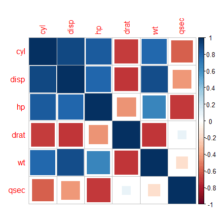
Corrplot is a graphical display for correlation matrix and confidence intervals. We can change the shape, layout, ordering, colour labels etc. using this powerful function. 

For corrplot, to work you need to install the corrplot package. The input to this function will be a correlation matrix. 

R Code - Visualization 

> #Generating the correlation matrix
> correlation <- cor(mtcars[2:7])
> correlation
            cyl       disp         hp        drat         wt        qsec
cyl   1.0000000  0.9020329  0.8324475 -0.69993811  0.7824958 -0.59124207
disp  0.9020329  1.0000000  0.7909486 -0.71021393  0.8879799 -0.43369788
hp    0.8324475  0.7909486  1.0000000 -0.44875912  0.6587479 -0.70822339
drat -0.6999381 -0.7102139 -0.4487591  1.00000000 -0.7124406  0.09120476
wt    0.7824958  0.8879799  0.6587479 -0.71244065  1.0000000 -0.17471588
qsec -0.5912421 -0.4336979 -0.7082234  0.09120476 -0.1747159  1.00000000
> 
> #Generating the plot
> corrplot(correlation)

> #Shape selection

> corrplot(correlation, method = "square")

> # Layout selection 

> corrplot(correlation, type = "lower")